Summary

I wish to shed some mild on advanced evaluation with out getting all of the technical particulars in the best way that are needed for the exact therapies that may be discovered in lots of wonderful commonplace textbooks.

Evaluation is about differentiation. Therefore, advanced differentiation might be my start line. It’s concurrently my end line as a result of its inverse, the advanced integration, is intently interwoven with advanced differentiation. By the shortage of particulars, I imply that I’ll typically assume a disc if a star-shaped area or a merely related open set could be adequate; or assume a differentiable operate if differentiability as much as finitely many factors would already be adequate. Additionally, the typically needed methods of gluing triangles for an integration path, or the epsilontic inside a area might be omitted.

The statements listed as theorems, nevertheless, might be exact. A few of them would possibly typically permit a wider vary of validity, i.e. extra generality. However, the reader will discover the essential concepts, definitions, tips, and theorems of the residue calculus; and if nothing else, see the place all of the ##pi##’s in integral formulation come from.

Complicated Differentiation

A operate ##f:Urightarrow V## is differentiable at ##x_0## if there’s a linear approximation ##D_{x_0}f=(Df)_{x_0}##, such that (Karl T.W. Weierstraß)
start{equation*}
f(x_0+v)=f(x_{0})+(D_{x_0}f)cdot v+r(v)
finish{equation*}
the place the error operate ##r## has the property, that it converges quicker to zero than linear in any path ##v##, which implies
$$lim_{v rightarrow 0}frac{r(v)}{v}=0.$$
If we rearrange this formulation, then
start{align*}
D_{x_0}f&= lim_{vto 0}D_{x_0}f = lim_{vto 0}left( dfrac{f(x_0+v)-f(x_0)}{v}-dfrac{r(v)}{v}proper)=lim_{vto 0} dfrac{f(x_0+v)-f(x_0)}{v}
finish{align*}
reveals the formulation that’s generally used to outline a by-product. It additionally exhibits that
$$
D_{x_0}f=(Df)_{x_0}=left. dfrac{df}{dx}proper|_{x_0}=f'(x_0)
$$
If ##f## is a operate of a one-dimensional vary, then the path ##v## can solely be a one-dimensional vector and we assume ##v=1## after we write
$$f'(x_0)=f'(x_0)cdot 1= D_{x_0}fcdot v.$$
The great thing about Weierstraß’s formulation lies in the truth that it carries all of the necessary properties of a by-product:

• locality:
  Weierstraß’s formulation requires validity in a area of ##x_0.##
• linear operator and Leibniz rule:
  ##D_{x_0}## is a derivation, i.e. ##D_{x_0}(alphacdot f+betacdot g)=alphacdot D_{x_0}(f) +betacdot D_{x_0}(g)## and ##D_{x_0}(fcdot g)=D_{x_0}(f)g(x_0)+f(x_0)D_{x_0}(g).##
• linearity:
  ##D_{x_0}f## is a linear operate, i.e. ##D_{x_0}f(alpha v+beta w)=alpha D_{x_0}f(v)+beta D_{x_0}f(w).##
• directionality, slope:
  A by-product ##(D_{x_0}f) v ## is directional, specifically the slope in path ##v.##
• approximation:
  ##r(v)=o(v).##

By permitting all elements ##x_0,f,v,r,D,D_{x_0},D_{x_0}f, D_{*}f## in Weierstraß’s formulation to be variables of an operator in its most basic which means, we instantly open the door to fiber bundles, world and native sections, differential types and tangent- in addition to cotangent bundles. Additionally word that we didn’t distinguish between actual and sophisticated features, but. This generality shall be our start line.

Each advanced linear operate ##varphi : mathbb{C}rightarrow mathbb{C}## is an actual linear operate, too, and will be written as
start{align*}
varphi(x+iy)&=underbrace{start{pmatrix}varphi_{11}&varphi_{12}varphi_{21}&varphi_{22}finish{pmatrix}}_{in mathbb{M}(2,mathbb{R})}(x+iy)=(varphi_{11}(x)+varphi_{12}(y))+i(varphi_{21}(x)+varphi_{22}(y))
finish{align*}
##mathbb{C}##-linearity signifies that
$$
(a+ib)varphi(x+iy)=varphi((ax-by)+i(bx+ay))
$$
and thus
start{align*}
(a+ib)&cdot (varphi_{11}(x)+varphi_{12}(y))+i(varphi_{21}(x)+varphi_{22}(y))
&=(varphi_{11}(ax)+varphi_{12}(ay)-varphi_{21}(bx)-varphi_{22}(by))
&phantom{=}+i(varphi_{11}(bx)+varphi_{12}(by)+varphi_{21}(ax)+varphi_{22}(ay))
&=(varphi_{11}(ax)-varphi_{11}(by)+varphi_{12}(bx)+varphi_{12}(ay))
&phantom{=}+i(varphi_{21}(ax)-varphi_{21}(by)+varphi_{22}(bx)+varphi_{22}(ay))
finish{align*}
Evaluating either side ends in
start{align*}
varphi_{11}=varphi_{22}, &textual content{ and } ,varphi_{21}+varphi_{12}=0quad (*)
finish{align*}
We all know that ##D_{z_0}## is a ##mathbb{C}##-linear operator, and ##D_{z_0}f## is a ##mathbb{C}##-linear operate. If we write ##f=u+iv## then
$$
D_{z_0}f=D_{z_0}u+iD_{z_0}v=left( left.dfrac{partial u}{partial x}proper|_{z_0}dx+left.dfrac{partial u}{partial y}proper|_{z_0}dyright)+ileft(left.dfrac{partial v}{partial x}proper|_{z_0}dx+left.dfrac{partial v}{partial y}proper|_{z_0}dyright)
$$
and our situation ##(*)## of ##mathbb{C}##-linearity turns into
$$
left. dfrac{partial u}{partial x }proper|_{z_0} = left. dfrac{partial v}{partial y}proper|_{z_0}textual content{ and }left. dfrac{partial u}{partial y}proper|_{z_0}+left. dfrac{partial v}{partial x}proper|_{z_0}=0,,
$$
the Cauchy-Riemann equations. Which means advanced differentiability is actual differentiability plus the Cauchy-Riemann equations. That is the principle distinction why advanced evaluation is greater than ##mathbb{R}^2## evaluation, advanced linearity.

Holomorphic Capabilities

We see by induction that skew-symmetric matrices with a relentless diagonal (spiral symmetry) maintain their construction if we multiply them by themselves
start{align*}
start{pmatrix}a&b-b&aend{pmatrix}^{n+1}&=start{pmatrix}c&d-d&cend{pmatrix}cdot start{pmatrix}a&b-b&aend{pmatrix}=start{pmatrix}ca-db&cb+da-da-cb&-db+caend{pmatrix}
finish{align*}
Meaning the Cauchy-Riemann property is invariant underneath exponentiation
$$
start{pmatrix}dfrac{partial u}{partial x}&dfrac{partial u}{partial y}[16pt] dfrac{partial v}{partial x}&dfrac{partial v}{partial y}finish{pmatrix}^n=start{pmatrix}dfrac{partial u}{partial x}&dfrac{partial u}{partial y}[16pt] -dfrac{partial u}{partial y}&dfrac{partial u}{partial x}finish{pmatrix}^n=
start{pmatrix}
pleft(dfrac{partial u}{partial x}, , ,dfrac{partial u}{partial y}proper) & qleft(dfrac{partial u}{partial x}, , ,dfrac{partial u}{partial y}proper) [16pt]
-qleft(dfrac{partial u}{partial x}, , ,dfrac{partial u}{partial y}proper) & pleft(dfrac{partial u}{partial x}, , ,dfrac{partial u}{partial y}proper)
finish{pmatrix}
$$
for some actual polynomials ##p(X,Y,n),q(X,Y,n)in mathbb{R}[X,Y].##

Definition: A fancy operate ##f:Urightarrow V## is holomorphic whether it is advanced differentiable in a non-empty, open, and related set ##U##, i.e. in a area. ##f## known as meromorphic whether it is holomorphic as much as a set of remoted factors, its poles. If ##f## is holomorphic on all the advanced airplane, then it’s referred to as an whole operate. An actual, or advanced operate is analytic at some extent ##z_0in U##, if there’s a energy sequence that converges to the operate worth in an open neighborhood of ##z_0##
$$
f(z)=sum_{n=0}^infty a_n(z-z_0)^n.
$$

Theorem: The next statements for ##f=u+iv, : ,Urightarrow V## are equal:

1. ##f## is advanced differentiable in a area ##U,## ##fin C^1(U).##
2. ##f## is bigoted usually advanced differentiable in a area ##U,## ##fin C^infty (U).##
3. ##f## is holomorphic on ##U,## ##fin mathcal{O}(U).##
4. The true and imaginary elements of ##f## are repeatedly actual differentiable and fulfill the Cauchy-Riemann partial differential equations (CR).
5. ##f## is analytic on ##U.##
6. ##f## is actual differentiable and ##{displaystyle {tfrac{partial f}{partial {bar {z}}}}:={tfrac{1}{2}} left({tfrac{partial }{partial x}} + i {tfrac{partial }{partial y}}proper)}(f) =0.##

Complicated Line Integrals

Now we have seen that the definition of advanced differentiation doesn’t require a change of actual differentiation, simply the reminder that the sphere ##mathbb{C}## which replaces the sphere ##mathbb{R}## will not be confused with the true vector house ##mathbb{R}^2.## We’re used to imagining advanced numbers as factors within the advanced airplane, however the advanced numbers will not be an actual airplane, they’re a one-dimensional advanced vector house over themselves.

The inverse operation is integration. And actual integration is the calculation of an oriented quantity, an space (quantity of the realm underneath the operate graph) within the case of a operate ##g:mathbb{R}rightarrow mathbb{R}.## Oriented signifies that we distinguish the areas above the ##x##-axis from the areas beneath the ##x##-axis, in addition to the mixing path from ##x=a## to ##x=b## from the mixing path from ##x=b## to ##x=a.## If the operate itself is a straight, say ##g(x)=r,## then the realm is that of a single rectangle
$$
int_a^b g(x),dx=int_a^b r,dx=[rx]_a^b=rb-ra=rcdot (b-a).
$$
If we proceed as above and solely substitute the true numbers with advanced numbers, then we get
start{align*}
int_{a+ic}^{b+id} g(x),dx&=int_{a+ic}^{b+id} (r+is),dz=[(r+is)z]_{a+ic}^{b+id}
&=(r(b-a)-s(d-c))+i(r(d-c)+s(b-a))
&=int_a^b r,dz +int_{ic}^{id}(is),dz+ int_{ic}^{id}r,dz+int_{a}^b (is),dz ,.
finish{align*}
Solely the variety of distinguishable orientations will increase as a result of ##i cdot i = -1## creates one other unfavourable space and imaginary volumes are allowed. This implies we now have to analyze the mixing path extra rigorously than simply from left to proper or from proper to left as we did in actual integration if we wish to perceive a posh quantity constructed by advanced lengths. Thankfully, the integral itself cares about all orientations so long as we don’t make an indication error, and so long as we’re not keen on an precise geometric quantity, that needed to be optimistic and actual.

To start with, we outline the apparent integral
$$
int_a^b f(t),dt := int_a^b u(t),dt +iint_a^b v(t),dt
$$
for (piecewise) steady features ##f=u+iv : mathbb{R}supset [a,b] rightarrow mathbb{C}.##

We additionally use this for the definition of the advanced line integral ##displaystyle{int_{z_1}^{z_2}f(z) ,dz}## the place we combine alongside a (actual) parameterized path ##gamma: [a,b] longrightarrow Gsubseteq mathbb{C}## from ##gamma (a)=z_1in G,gamma (b)=z_2in G## for a posh operate ##f: Glongrightarrow mathbb{C}## outlined on a area ##Gsubseteq mathbb{C}##
start{align*}
int_gamma f(z),dz &=…textual content{ (substitution }z=gamma(t), , ,dz=gamma’,dt)
…&=int_a^b (fcirc gamma )(t)cdot gamma’,dt =int_a^b f(gamma (t))cdot gamma'(t),dt
finish{align*}
The advanced line integral will depend on a priori on the mixing path! This could simply be proven for ##f(z)=bar{z}.## Nevertheless, if ##f## is holomorphic, then its line integrals are path impartial.

Cauchy’s Integral Theorem: If ##f:Glongrightarrow mathbb{C}## is a steady advanced operate then ##f## has an anti-derivative on ##G## if and provided that ##displaystyle{oint_gamma f(z),dz=0}## for any closed integration path ##gamma## in ##G##, ##gamma(a)=z_0=gamma(b).##

Each is true for a star-shaped area ##G,## e.g. a convex area, and a holomorphic operate ##f.##

Instance: Take into account the border ##gamma(t)=z_0+re^{i t}, , ,0leq tleq 2pi## of the disc ##G=D_r(z_0)## round a central level ##z_0.## Then
start{align*}
oint_gamma dfrac{1}{z-z_0},dz&=int_0^{2pi}dfrac{1}{re^{it}} cdot ire^{it} ,dt=icdot int_0^{2pi}dt=2pi i
oint_gamma left(z-z_0right)^p,dz&stackrel{(pneq -1)}{=}int_0^{2pi} r^p e^{i p t} cdot ire^{it},dt=ir^{p+1}int_0^{2pi} e^{i(p+1)t},dt
&=ir^{p+1}left[dfrac{e^{i(p+1)t}}{i(p+1)}right]_0^{2pi}=dfrac{r^{p+1}}{p+1}(e^{2(p+1)pi i t}-e^0)=0,.
finish{align*}
Therefore, we get the necessary formulation
$$
oint_gamma left(z-z_0right)^p,dz=start{circumstances}
2pi i & textual content{ if } p = -1
0 & textual content{ if } pneq -1 ,.
finish{circumstances}
$$

Corollary: If ##Dsubset mathbb{C}## is a disc, and ##zin mathbb{C} backslash partial D## then
$$
oint_{partial D} ,dfrac{dzeta}{zeta -z}=start{circumstances}
2pi i & textual content{ if } zin D
0 & textual content{ else } ,.
finish{circumstances}
$$

Complicated Integration

If ##f:Grightarrow mathbb{C}## is holomorphic, then
$$
f(zeta)=f(z)+underbrace{left( (D_{z}f)+underbrace{dfrac{r(zeta-z)}{zeta-z}}_{stackrel{zeta to z}{longrightarrow };;0} proper)}_{=:Delta_z(zeta)}cdot (zeta-z)
$$
with an all over the place steady and in addition to ##z## even holomorphic operate ##Delta_z.## Thus
start{align*}
0&=oint_{partial D}Delta(zeta),dzeta =oint_{partial D}dfrac{f(zeta)-f(z)}{zeta -z},dzeta
&=oint_{partial D}dfrac{f(zeta)}{zeta -z},dzeta – f(z) oint_{partial D}dfrac{1}{zeta -z},dzeta =oint_{partial D}dfrac{f(zeta)}{zeta -z},dzeta – f(z)cdot 2pi i
finish{align*}
and
$$
f(z)=dfrac{1}{2pi i}oint_{partial D}dfrac{f(zeta)}{zeta -z},dzeta
$$
We even have

Theorem: The next statements for ##f=u+iv, : ,Urightarrow V## are equal:

1. ##f## is holomorphic on ##U.##
2. ##f## is steady and its path integral over any closed, contractible path vanishes.
3. The operate values of ##f## on the inside of a disc ##Dsubseteq U## will be decided by the operate values on the border of this disc by
   Cauchy’s integral formulation
   $$ f(z)=dfrac{1}{2pi i} oint_{partial D} dfrac{f(zeta)}{zeta – z},dzeta,.$$

Allow us to now introduce the trick with the geometric sequence. ##f:Drightarrow mathbb{C}## be a steady operate an a compact set ##D, , , z_0notin D ## and ##R=operatorname{dist}(z_0,D).## Then
start{align*}
dfrac{1}{zeta – z}&=dfrac{1}{(zeta -z_0)-(z-z_0)}=dfrac{1}{zeta -z_0}cdot dfrac{1}{1-dfrac{z-z_0}{zeta-z_0}}=dfrac{1}{zeta -z_0}cdot sum_{n=0}^infty left(dfrac{z-z_0}{zeta-z_0}proper)^n
finish{align*}
for ##|z-z_0|<Rleq |zeta-z_0|## and ##zin D_R(z_0), , ,zeta in D.## Since ##f## is bounded on the compact set ##D,## say ##0<|f(zeta)|<C,## we now have
$$
left| dfrac{f(zeta)}{(zeta-z_0)^{n+1}}cdot(z-z_0)^n proper|leq dfrac{C}{R}cdot left(dfrac{z-z_0}{R}proper)^n
$$
and the sequence on the fitting converges for any fastened ##zin D_R(z_0).## Thus
$$
dfrac{f(zeta)}{zeta – z}=dfrac{f(zeta)}{zeta -z_0}cdot sum_{n=0}^infty left(dfrac{z-z_0}{zeta-z_0}proper)^n=sum_{n=0}^infty dfrac{f(zeta)}{(zeta-z_0)^{n+1}}cdot (z-z_0)^n
$$
converges completely and uniformly for a hard and fast ##z## for ##zeta in D## by Weierstraß’s criterion. Lastly,
start{align*}
f(z)=dfrac{1}{2pi i}oint_gamma dfrac{f(zeta)}{zeta – z},dzeta= sum_{n=0}^infty underbrace{left(dfrac{1}{2pi i} oint_gamma dfrac{f(zeta)}{(zeta-z_0)^{n+1}},dzeta proper)}_{=:a_n}cdot (z-z_0)^n
finish{align*}
converges absolute and uniformly on the inside of ##D_R(z_0)## versus the all over the place holomorphic, and by building analytic operate
$$
f(z)=sum_{n=0}^infty a_n(z-z_0)^n,.
$$
If we apply this to the border of a disc ##gamma(t)=z_0+re^{it}## with ##0<r<R## and ##0leq tleq 2pi ,## we get

Cauchy’s Growth Theorem: Let ##f:Grightarrow mathbb{C}## be a posh, holomorphic operate on a area ##G## and ##z_0in G.## Let additional be ##R## the maximal radius of an open disc round ##z_0## that matches into ##G.## Then there’s a energy sequence
$$
f(z)=sum_{n=0}^infty a_n(z-z_0)^n,
$$
that converges for all ##0<r<R## on the disc ##D_r(z_0)## completely and uniformly versus ##f(z).## For each such ##r## is
$$
displaystyle{a_n=dfrac{1}{2pi i} oint_{partial D_r(z_0)} dfrac{f(zeta)}{(zeta-z_0)^{n+1}},dzeta}
$$
and ##f## is on ##G## arbitrary usually advanced differentiable.

Residue Theorem

Allow us to begin with Laurent’s decomposition trick for a holomorphic operate ##f:mathcal{R}rightarrow mathbb{C}## on a hoop ##mathcal{R}={zin mathbb{C},|,0<r<|z|<R}.## There exists a decomposition
$$
f(z)=g(z)+hleft(dfrac{1}{z}proper)
$$
into holomorphic features on discs
$$
g:D_R(0)rightarrow mathbb{C}; , ;h:D_{1/r}(0)rightarrow mathbb{C}
$$
The decomposition turns into distinctive if we require ##h(0)=0.## Since holomorphic features are analytic, we now have an enlargement into energy sequence
$$
f(z)= sum_{n=0}^infty a_nz^n+sum_{n=0}^infty b_nleft(dfrac{1}{z}proper)^n=sum_{n=-infty }^infty c_nz^n
$$
For an enlargement at ##z_0## we obtain a Laurent sequence ##(r<rho<R)##
$$
f(z)=sum_{n=-infty }^infty a_n (z-z_0)^n; , ;a_n=displaystyle{dfrac{1}{2pi i} oint_{partial D_rho(z_0)} dfrac{f(zeta)}{(zeta-z_0)^{n+1}},dzeta}
$$
Observe that ##r=0,R=infty ,## and ##r=R## are potential settings. These radii will be calculated by the formulation of Cauchy-Hadamard
$$
r=limsup_{nto infty } sqrt[n]{|a_{-n}|}; , ;R=dfrac{1}{displaystyle{limsup_{nto infty } sqrt[n]{|a_{n}|}}}
$$
Definition: Let ##f:Grightarrow mathbb{C}## be a holomorphic operate that doesn’t fully vanish on the area ##Gsubseteq mathbb{C}.## The coefficient at ##-1##
$$
operatorname{Res}_{z_0}(f)=a_{-1}=dfrac{1}{2pi i} oint_{partial D_rho(z_0)} f(zeta) ,dzeta
$$
known as the residue of ##f## at ##z_0.## It’s the solely coefficient with no ##z-z_0## time period within the Laurent sequence of ##f.##

A degree ##z_0## known as a zero of order ##m## if there’s a holomorphic operate ##g:D_r(z_0)rightarrow mathbb{C}## such that
$$
f(z)=(z-z_0)^m g(z); , ;g(z_0)neq 0 .
$$
A degree ##z_0## known as a pole (remoted singularity) of order ##m## if there’s a holomorphic operate ##g:D_r(z_0)rightarrow mathbb{C}## such that
$$
f(z)=(z-z_0)^{-m}g(z); , ;g(z_0)neq 0 .
$$
A pole is a zero of ##1/f.## The residue of a pole of order ##m## is
$$
operatorname{Res}_{z_0}(f)= dfrac{1}{(n-1)!} lim_{zto z_0}{dfrac{d^{n-1}}{dz^{n-1}}} left((z-z_0)^{n}f(z)proper)
$$
Now we have seen that surrounding a disc as soon as means ##;dfrac{1}{2pi i}displaystyle{oint_{partial D} ,dfrac{dzeta}{zeta -z}}=1.##

If we as a substitute have any closed curve ##gamma ## round ##z_0,## then we outline the winding variety of ##gamma ## round ##z_0## as
$$
operatorname{Ind}_gamma (z_0):=dfrac{1}{2pi i}oint_{gamma} ,dfrac{dzeta}{zeta -z}.
$$

Residue Theorem: Let ##f:Grightarrow mathbb{C}## be a holomorphic features as much as finitely many remoted singularities ##z_1,ldots,z_q,## i.e. ##f## is meromorphic, and ##gamma ## a closed, piecewise clean curve within the area ##G,## then
$$
oint_gamma f(z),dz=2pi i sum_{ok=1}^q operatorname{Ind}_gamma (z_k) operatorname{Res}_{z_k}(f)
$$
Let’s name the set of zeros ##Z## and the set of poles ##P## of a meromorphic operate ##f,## and require that our integration path ##gamma ## doesn’t comprise any of them. We have already got seen that we are able to write ##f(z) =(z-z_0)^{m}g(z) = (z-z_0)^{operatorname{ord}_{z_0}(f)}## for any ##z_0in Zcup P## of order ##|m|.## Then
$$
dfrac{f'(z)}{f(z)}=dfrac{m}{z-z_0}+dfrac{g'(z)}{g(z)}.
$$
##dfrac{g'(z)}{g(z)}## is holomorphic at ##z_0## since ##g(z_0)neq 0.## The residue of ##f’/f## at ##z_0## equals subsequently precisely the order ##m## of the zero or pole ##z_0## of ##f## and
$$
dfrac{1}{2pi i}oint_gamma dfrac{f'(z)}{f(z)},dz=sum_{z_0in Zcup P} operatorname{Ind}_gamma (z_0)cdot operatorname{Res}_{z_0}left(dfrac{f’}{f}proper) =sum_{z_0in Zcup P} operatorname{Ind}_gamma (z_0)cdot operatorname{ord}_{z_0}(f)
$$
the place
$$
operatorname{Res}_{z_0}left(dfrac{f’}{f}proper) = operatorname{ord}_{z_0}(f)=
start{circumstances}
ok & textual content{if } z_0 in Z textual content{ of order ok }
-k & textual content{if } z_0 in P textual content{ of order ok }
0 & textual content{ else }
finish{circumstances}
$$

Properties of Residues

Cauchy’s integral theorem says that ##operatorname{Res}_{z_0}(f)=0## for a holomorphic operate ##f:Grightarrow mathbb{C}## and ##z_0in G.## Let’s see how residues will be calculated in different circumstances. Say ##z_m## is a zero of order ##m## and ##p_m## a pole of order ##m## of a meromorphic operate ##f:Grightarrow mathbb{C}.## Let additional be ##h:Grightarrow mathbb{C}## holomorphic at these factors, and ##g## one other meromorphic operate. Then ##operatorname{Res}_{z_0}## is ##mathbb{C}##-linear and

$$
start{array}{ll}
operatorname{Res}_{z_0}(alpha f+beta g)=alphaoperatorname{Res}_{z_0}(f)+betaoperatorname{Res}_{z_0}(g) &(z_0in G , , ,alpha, beta in mathbb{C}) [16pt]
operatorname{Res}_{z_1}left(dfrac{h}{f}proper)=dfrac{h(z_1)}{f'(z_1)}&
operatorname{Res}_{z_1}left(dfrac{1}{f}proper)=dfrac{1}{f'(z_1)}[16pt]
operatorname{Res}_{z_m}left(hdfrac{f’}{f}proper)=h(z_m)cdot m&operatorname{Res}_{z_m}left(dfrac{f’}{f}proper)=m[16pt]
operatorname{Res}_{p_1}(hcdot f)=h(p_1)cdot operatorname{Res}_{p_1}(f)&operatorname{Res}_{p_1}(f)=displaystyle{lim_{z to p_1}((z-p_1)f(z))}[16pt]
operatorname{Res}_{p_m}(f)=dfrac{1}{(m-1)!}displaystyle{lim_{z to p_m}dfrac{partial^{m-1} }{partial z^{m-1}}left( (z-p_m)^m f(z) proper)}&operatorname{Res}_{p_m}left(dfrac{f’}{f}proper)=-m[16pt]
operatorname{Res}_{infty }(f)=operatorname{Res}_0left(-dfrac{1}{z^2}fleft(dfrac{1}{z}proper)proper)&operatorname{Res}_{p_m}left(hdfrac{f’}{f}proper)=-h(p_m)cdot m[16pt]
operatorname{Res}_{z_0}(h)=0 & operatorname{Res}_0left(dfrac{1}{z}proper)=1[16pt]
operatorname{Res}_1left(dfrac{z}{z^2-1}proper)=operatorname{Res}_{-1}left(dfrac{z}{z^2-1}proper)=dfrac{1}{2}&operatorname{Res}_0left(dfrac{e^z}{z^m}proper)=dfrac{1}{(m-1)!}
finish{array}
$$

Actual Integration with Residues

Take into account an actual rational operate ##f:mathbb{R}rightarrow mathbb{R}## with ##deg(f)leq -2## that has no poles on the true axis.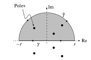

We wish to combine ##f## alongside the true axis, however take this as part of the advanced airplane. Our major integration path is a composite of the true path ##gamma :[-r,r]rightarrow [-r,r]subseteq mathbb{C}, , ,gamma(t)=t## and the advanced path ##tilde{gamma }:[0,pi]rightarrow mathbb{C}, , ,tilde{gamma }(t)=re^{it}## within the higher half of the airplane the place ##mathfrak{Im}(z)geq 0.## The residue theorem says

$$
displaystyle{oint_{gamma oplus tilde{gamma }}f(z),dz =int_gamma f(z),dz +int_{tilde{gamma }}f(z),dz= 2pi isum_{ok=1}^qoperatorname{Res}_{z_k}(f). }
$$
and all poles of ##f## lie inside our closed integration path so long as the radius ##r## is massive sufficient. Furthermore, for any normed, i.e. the main coefficient equals ##1##, advanced polynomial ##P(z)## of diploma ##n## there’s an ##Rin mathbb{R}^+## such that for all ##zin mathbb{C}## with ##|z|geq R##
$$
dfrac{1}{2}|z|^nleq |P(z)|leq dfrac{3}{2}|z|^n
$$
which will be confirmed with the triangle inequalities. We get for our rational operate that there’s a optimistic actual fixed ##cin mathbb{R}^+## such that (##L##= size)
$$
displaystyle{left|int_{tilde{gamma }}f(z),dzright|leq L(gamma )cdot max_=r|f(z)|leq pi r cdot cr^{-2}=pidfrac{c}{r};stackrel{rto infty }{longrightarrow };0}
$$
Therefore
start{align*}
int_{-infty }^infty f(x),dx&= displaystyle{lim_{r to infty} int_{-r}^rf(x),dx}=displaystyle{lim_{r to infty} int_gamma f(z),dz +0}
&=displaystyle{lim_{r to infty} int_gamma f(z),dz + lim_{r to infty}int_{tilde{gamma }}f(z),dz }= 2pi isum_{ok=1}^qoperatorname{Res}_{z_k}(f).
finish{align*}

Instance: We wish to discover ##displaystyle{int_{-infty }^infty dfrac{dx}{(1+x^2)^n}}## for a optimistic integer ##nin mathbb{N}## which equals ##2pi i operatorname{Res}_{i}(f)## for the meromorphic operate $$f(x)=dfrac{1}{(z^2+1)^n}=dfrac{1}{(z+i)^n(z-i)^n}$$ that has ##z=i## as solely pole of order ##n## within the higher half of the advanced airplane.
start{align*}
operatorname{Res}_{i}left(dfrac{1}{(1+z^2)^n}proper)&=dfrac{1}{(n-1)!}displaystyle{;lim_{z to i}};dfrac{partial^{n-1}}{partial z^{n-1}}left((z-i)^ndfrac{1}{(1+z^2)^n}proper)
&=dfrac{1}{(n-1)!}displaystyle{;lim_{z to i}};dfrac{partial^{n-1}}{partial z^{n-1}}(z+i)^{-n}
&=dfrac{1}{(n-1)!}displaystyle{;lim_{z to i}
(-n)(-n-1)cdots (-2n+2)(z+i)^{-2n+1}}
&=dfrac{1}{(n-1)!}(-1)^{n-1}dfrac{(2n-2)!}{(n-1)!}(2i)^{-2n+1}=-dfrac{i}{2^{-2n+1}}binom{2n-2}{n-1}
finish{align*}
and
$$
displaystyle{int_{-infty }^infty dfrac{dx}{(1+x^2)^n}= dfrac{pi}{2^{2n-2}}}binom{2n-2}{n-1}.
$$
It may be confirmed by related strategies as above that (cp. Fourier remodel)
$$
int_{-infty }^infty f(x)e^{ix},dx=2pi i sum_{ok=1}^qoperatorname{Res}_{z_k}left(f(z)e^{iz}proper)
$$
for an actual rational operate ##f## with ##deg(f)leq -2## and poles ##z_1,ldots,z_q## on the strict higher half of the advanced airplane, i.e. ##mathfrak{Im}(z_k)>0.##

Instance:

start{align*}
int_{-infty }^infty dfrac{cos x}{1+x^2},dx&=mathfrak{Re}left(int_{-infty }^infty dfrac{frac{1}{2}(e^{ix}+e^{-ix})}{1+x^2},dx proper)=mathfrak{Re}left(int_{-infty }^infty dfrac{e^{ix}}{1+x^2},dxright)
&=mathfrak{Re}left(2pi i operatorname{Res}_{i}left(dfrac{e^{iz}}{1+z^2}proper)proper)=mathfrak{Re}left(2pi i displaystyle{;lim_{z to i}}(z-i)dfrac{e^{iz}}{1+z^2} proper)
&=mathfrak{Re}left(2pi i cdot dfrac{e^{-1}}{(i+i)}proper)=dfrac{pi}{e}
finish{align*}
These methods are used to show the marginally extra basic

Jordan’s Lemma: Let ##f(z)=e^{ialpha z}g(z):mathbb{C}longrightarrow mathbb{C}## be a complex-valued, steady operate with ##alphain mathbb{R}^+## and ##gamma :[0,pi]rightarrow mathbb{C}, , ,gamma(t)=re^{it}, , ,rin mathbb{R}^+.## Then
$$
left| int_{gamma } f(z) , dz proper| =left| int_{gamma } e^{ialpha z}g(z) , dz proper|le frac{pi}{alpha} M_r quad textual content{the place} quad M_r := max_{t in [0,pi]} left| g left(r e^{i t}proper) proper|.
$$
We get particularly for features ##g## with a uniform convergence ##displaystyle{lim_ to inftyg(z)=0}## for ##zin {zin mathbb,mathfrak{Im}(z)>0}## that
$$
displaystyle{lim_{r to infty}int_gamma f(z),dz =lim_{r to infty}int_gamma e^{ialpha z}g(z),dz=0}
$$
That is additionally true for ##alpha=0## if ##displaystyle{lim_ to inftyzcdot g(z)=0}.##

Some extra examples that may be calculated by these strategies are

start{align*}
int_{-infty }^infty dfrac{cos (alpha x)}{1+x^2},dx=dfrac{pi}{e^alpha}; &, ; int_{-infty }^infty dfrac{xsin (alpha x)}{1+x^2},dx=dfrac{pi}{e^alpha} [6pt]
int_0^infty dfrac{1}{1+x^3},dx = dfrac{2pi}{3sqrt{3}}; &, ;int_0^infty dfrac{1}{4+x^4},dx = dfrac{pi}{8}[6pt]
int_{-infty }^infty dfrac{1}{e^x+e^{-x}},dx =dfrac{pi }{2}; &, ;int_{-infty }^infty dfrac{x}{e^x-e^{-x}},dx =dfrac{pi^2 }{4}
finish{align*}

Sources