
[ad_1]
A typical process in evaluation is to acquire bounds on sums

or integrals

the place 


or

the place we use 


or
the place 


the place 
Listed here are some typical examples of such estimation issues, drawn from latest questions on MathOverflow:
In comparison with different estimation duties, corresponding to that of controlling oscillatory integrals, exponential sums, singular integrals, or expressions involving a number of unknown capabilities (which are solely identified to lie in some operate areas, corresponding to an 
Considerably within the spirit of this earlier put up on evaluation downside fixing methods, I’m going to strive right here to gather some common rules and methods that I’ve discovered helpful for these types of issues. As with the earlier put up, I hope this shall be one thing of a residing doc, and encourage others so as to add their very own suggestions or options within the feedback.
— 1. Asymptotic arithmetic —
Asymptotic notation is designed in order that most of the standard guidelines of algebra and inequality manipulation proceed to carry, with the caveat that one must be cautious if subtraction or division is concerned. For example, if one is aware of that 


and extra usually we’ve the triangle inequality

(Once more, we stress that this kind of rule implicitly requires the 
One other rule of inequalities that’s inherited by asymptotic notation is that if one has two bounds

for an identical quantity
That is an instance of a “free transfer”: a substitute of bounds that doesn’t lose any of the energy of the unique bounds, since in fact (2) implies (1). In distinction, different methods to mix the 2 bounds (1), corresponding to taking the geometric imply
whereas usually handy, are usually not “free”: the bounds (1) indicate the averaged certain (3), however the certain (3) doesn’t indicate (1). Alternatively, the inequality (2), whereas it doesn’t concede any logical energy, can require extra calculation to work with, actually because one finally ends up splitting up instances corresponding to 
For example, suppose one wished to indicate that the sum
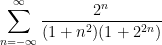
was convergent. Decrease bounding the denominator time period 


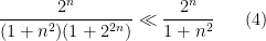
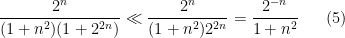
so by making use of (2) we get hold of the unified certain

To cope with this certain, we will break up into the 2 contributions 


is totally convergent, and within the latter case we see that the sum

can be completely convergent, so all the sum is totally convergent. However as soon as one has this argument, one can attempt to streamline it, as an illustration by taking the geometric imply of (4), (5) slightly than the minimal to acquire the weaker certain

and now one can conclude with out decomposition simply by observing absolutely the convergence of the doubly infinite sum 
One of many key benefits of coping with order of magnitude estimates, versus sharp inequalities, is that the arithmetic turns into tropical. Extra explicitly, we’ve the necessary rule
whenver

In praticular, if 


or not less than an higher certain
of 


The above divide and conquer technique doesn’t straight apply when one is decomposing into an unbounded variety of items 


that appears promising for the issue, then it will suffice to acquire exponentially decaying bounds corresponding to

for all 


due to the geometric collection system. (Right here it will be important that the implied constants within the asymptotic notation are uniform on 


would already be enough, though harmonic decay such

isn’t fairly sufficient (the sum 
for all 


Typically, when attempting to show an estimate corresponding to

(the place 


— 1.1. Psychological distinctions between actual and asymptotic arithmetic —
The adoption of the “divide and conquer” technique requires a sure psychological shift from the “simplify, simplify” technique that one is taught in highschool algebra. Within the latter technique, one tries to gather phrases in an expression make them as brief as doable, as an illustration by working with a standard denominator, with the concept that unified and elegant-looking expressions are “less complicated” than sprawling expressions with many phrases. In distinction, the divide and conquer technique is deliberately extraordinarily keen to tremendously enhance the whole size of the expressions to be estimated, as long as every particular person element of the expressions seems simpler to estimate than the unique one. Each methods are nonetheless attempting to scale back the unique downside to an easier downside (or assortment of less complicated sub-problems), however the metric by which one judges whether or not the issue has change into less complicated is slightly completely different.
A associated psychological shift that one must undertake in evaluation is to maneuver away from the precise identities which are so prized in algebra (and in undergraduate calculus), because the precision they provide is commonly pointless and distracting for the duty at hand, and infrequently fail to generalize to extra sophisticated contexts wherein actual identities are now not obtainable. As a easy instance, think about the duty of estimating the expression

the place 


and

one can mix them utilizing (2) to acquire the higher certain
and comparable arguments additionally give the matching decrease certain, thus

This certain, whereas cruder than the precise reply of

for which there isn’t any closed type actual expression when it comes to elementary capabilities such because the arctangent.
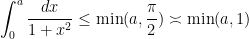
As a common rule, as a substitute of relying completely on actual formulae, one ought to search approximations which are legitimate as much as the diploma of precision that one seeks within the last estimate. For example, suppose one one needs to determine the certain

for all small enough 

which one can invert utilizing the geometric collection system 
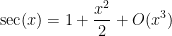
from which the declare follows. (One might even have computed the Taylor enlargement of 

for small

to the sine operate that’s correct to order
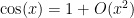
to the cosine operate that’s correct to order 

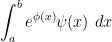
Alternatively, some actual formulae are nonetheless very helpful, significantly if the tip results of that system is clear and tractable to work with (versus involving considerably unique capabilities such because the arctangent). The geometric collection system, as an illustration, is an especially useful actual system, a lot in order that it’s usually fascinating to manage summands by a geometrical collection purely to make use of this system (we already noticed an instance of this in (7)). Precise integral identities, corresponding to
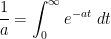
or extra usually

for 


every time 
![{f: [a-1,b+1] rightarrow {bf R}}](https://s0.wp.com/latex.php?latex=%7Bf%3A+%5Ba-1%2Cb%2B1%5D+%5Crightarrow+%7B%5Cbf+R%7D%7D&bg=ffffff&fg=000000&s=0&c=20201002)

every time 
![{f: [a,b] rightarrow {bf R}}](https://s0.wp.com/latex.php?latex=%7Bf%3A+%5Ba%2Cb%5D+%5Crightarrow+%7B%5Cbf+R%7D%7D&bg=ffffff&fg=000000&s=0&c=20201002)
Train 1 Suppose
obeys the quasi-monotonicity property
every time
. Present that
for any integers
.
Train 2 Use (11) to acquire the “low cost Stirling approximation”
for any pure quantity
. (Trace: take logarithms to transform the product
right into a sum.)

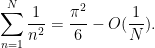
With follow, it is possible for you to to establish any time period in a computation which is already “negligible” or “acceptable” within the sense that its contribution is at all times going to result in an error that’s smaller than the specified accuracy of the ultimate estimate. One can then work “modulo” these negligible phrases and discard them as quickly as they seem. This will help take away loads of muddle in a single’s arguments. For example, if one needs to determine an asymptotic of the shape
for some most important time period 
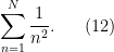
This can be a partial sum for the zeta operate

so it might make sense so as to add and subtract the tail 
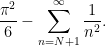
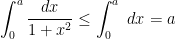
To cope with the tail, we change from a sum to the integral utilizing (10) to certain
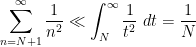
giving us the moderately correct certain
One can sharpen this approximation considerably utilizing (11) or the Euler–Maclaurin system; we depart this to the reader.
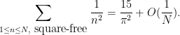
One other psychological shift when switching from algebraic simplification issues to estimation issues is that one must be ready to let go of constraints in an expression that complicate the evaluation. Suppose as an illustration we now want to estimate the variant
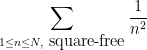
of (12), the place we are actually limiting
in order earlier than we will write the specified expression as

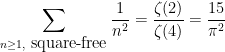
Beforehand, we utilized the integral take a look at (10), however this time we can’t achieve this, as a result of the restriction to square-free integers destroys the monotonicity. However we will merely take away this restriction:

Heuristically not less than, this transfer solely “prices us a relentless”, since a optimistic fraction (
— 2. Extra on decomposition —
The way in which wherein one decomposes a sum or integral corresponding to 


If an expression includes a distance 


when it comes to the 2 actual parameters 

- (i) The area the place
.
- (ii) The area the place
.
- (iii) The area the place
.
(This isn’t the one method to lower up the integral, however it’s going to suffice. Usually there isn’t any “canonical” or “elegant” method to carry out the decomposition; one ought to simply attempt to discover a decomposition that’s handy for the issue at hand.)
The explanation why we need to carry out such a decomposition is that in every of the three instances, one can simplify how the integrand depends upon 


Utilizing a variant of (9), this expression is akin to

The contribution of area (ii) could be dealt with equally, and can be akin to (14). Lastly, in area (iii), we see from the triangle inequality that 
Now that we’ve centered the integral round 

On the one hand this integral is bounded by
and then again we will certain

and so we will certain the contribution of (iii) by 


A robust and customary sort of decomposition is dyadic decomposition. If the summand or integrand includes some amount 


into dyadic items
after which search to estimate every dyadic block 
because the summand 

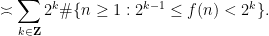
This now converts the issue of estimating the sum (15) to the extra combinatorial downside of estimating the scale of the dyadic degree units 

the place 

Train 3 Let
be a easy compact submanifold of
. Set up the certain
for all
, the place the implied constants are allowed to rely on
. (This may be achieved both by a vertical dyadic decomposition, or a dyadic decomposition of the amount
.)

Train 4 Remedy downside (ii) from the introduction to this put up by dyadically decomposing within the
variable.
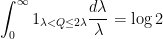
Comment 5 By such instruments as (10), (11), or Train 1, one might convert the dyadic sums one obtains from dyadic decomposition into integral variants. Nevertheless, if one wished, one might “lower out the middle-man” and work with steady dyadic decompositions slightly than discrete ones. Certainly, from the integral id
for any
, along with the Fubini–Tonelli theorem, we get hold of the continual dyadic decomposition
for any amount
that’s optimistic every time
parameter which might be difficult to execute if this have been a discrete variable.

— 3. Exponential weights —
Many sums contain expressions which are “exponentially massive” or “exponentially small” in some parameter. A primary rule of thumb is that any amount that’s “exponentially small” will seemingly give a negligible contribution when put next towards portions that aren’t exponentially small. For example, if an expression includes a time period of the shape 
for some 


To make such a heuristic exact, one can carry out a dyadic decomposition within the exponential weight 
Train 6 Use this decomposition to carefully set up the certain
for any

Train 7 Remedy downside (i) from the introduction to this put up.
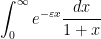
Extra usually, if one is working with a sum or integral corresponding to

or

with some exponential weight 


for 
we will rewrite this as
The exponential weight 


for 

giving the asymptotic

for
Train 8 Within the converse course, set up the higher certain
for some absolute fixed
Train 9 If
for some
, present that
(Trace: estimate the ratio between consecutive binomial coefficients
after which management the sum by a geometrical collection).

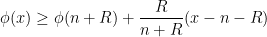
When the utmost of the exponent
the place 
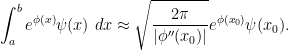
The heuristic justification is as follows. The primary contribution must be when

since at a non-degenerate most we’ve 


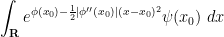
which could be computed to equal 
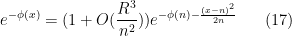
Allow us to illustrate how this argument could be made rigorous by contemplating the duty of estimating the factorial 
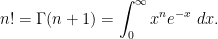
As 

the place
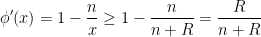
The operate 


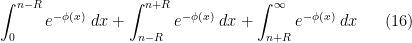
the place 
The primary time period is predicted to be the center time period, so we will use crude strategies to certain the opposite two phrases. For the primary half the place 

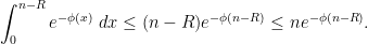
(We anticipate 


for
and after a brief calculation this offers

Now we flip to the necessary center time period. If we assume 


If we assume that 
for
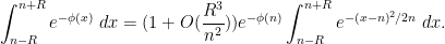
If we additionally assume that 

Placing all this collectively, and utilizing eqref for particulars.
Train 10 Remedy downside (iii) from the introduction. (Trace: extract out the time period
to jot down because the exponential issue
, inserting all the opposite phrases (that are of polynomial measurement) within the amplitude operate
. The operate
; carry out a Taylor enlargement and mimic the arguments above.)
[ad_2]