
[ad_1]
Terry Rudolph, PsiQuantum & Imperial Faculty London
Throughout a latest go to to the wild western city of Pasadena I bought right into a shootout at high-noon attempting to elucidate the nuances of this query to a colleague. Here’s a extra thorough (and fewer dangerous) try to get better!
tl;dr Photonic quantum computer systems can carry out a helpful computation orders of magnitude sooner than a superconducting qubit machine. Surprisingly, this might nonetheless be true even when each bodily timescale of the photonic machine was an order of magnitude longer (i.e. slower) than these of the superconducting one. However they gained’t be.
SUMMARY
- There’s a false impression that the gradual price of entangled photon manufacturing from many present (“postselected”) experiments is one way or the other related to the logical velocity of a photonic quantum pc. It isn’t, as a result of these experiments don’t use an optical swap.
- If we care about how briskly we will resolve helpful issues then photonic quantum computer systems will finally win that race. Not solely as a result of in precept their parts can run sooner, however due to basic architectural flexibilities which imply they should do fewer issues.
- In contrast to most quantum programs for which related bodily timescales are decided by “constants of nature” like interplay strengths, the related photonic timescales are decided by “classical speeds” (optical swap speeds, digital sign latencies and so forth). Surprisingly, even when these had been slower – which there is no such thing as a cause for them to be – the photonic machine can nonetheless compute sooner.
- In a easy world the velocity of a photonic quantum pc would simply be the velocity at which it’s potential to make small (fastened sized) entangled states. GHz charges for such are believable and correspond to the a lot slower MHz code-cycle charges of a superconducting machine. However we wish to leverage two distinctive photonic options: Availability of lengthy delays (e.g. optical fiber) and ease of nonlocal operations, and as such the general story is far much less easy.
- If what floats your boat are actually gradual issues, like chilly atoms, ions and so forth., then the hybrid photonic/matter structure outlined right here is the best way you possibly can construct a quantum pc with a sooner logical gate velocity than (say) a superconducting qubit machine. You ought to be throughout it.
- Magnifying the variety of logical qubits in a photonic quantum pc by 100 may very well be achieved just by making optical fiber 100 occasions much less lossy. There are causes to imagine that such fiber is feasible (although not straightforward!). This is only one instance of the “photonics is totally different, photonics is totally different, ” mantra we must always all chant each morning as we stagger away from bed.
- The pliability of photonic architectures means there’s far more unexplored territory in quantum algorithms, compiling, error correction/fault tolerance, system architectural design and far more. Should you’re a scholar you’d be mad to work on anything!
Sorry, I understand that’s form of an in-your-face checklist, a few of which is clearly simply my opinion! Lets see if I could make it yours too 🙂
I’m not going to reiterate all the usual stuff about how photonics is nice due to how manufacturable it’s, its excessive temperature operation, straightforward networking modularity blah blah blah. That story has been informed many occasions elsewhere. However there are subtleties to understanding the eventual computational velocity of a photonic quantum pc which haven’t been defined fastidiously earlier than. This put up goes to slowly lead you thru them.
I’ll solely be speaking about helpful, large-scale quantum computing – by which I imply machines able to, at a minimal, implementing billions of logical quantum gates on tons of of logical qubits.
PHYSICAL TIMESCALES
In a quantum pc constructed from matter – say superconducting qubits, ions, chilly atoms, nuclear/digital spins and so forth, there’s at all times a minimum of one pure and inescapable timescale to level to. This sometimes manifests as some discrete vitality ranges within the system, the degrees that make the 2 states of the qubit. Associated timescales are decided by the interplay strengths of a qubit with its neighbors, or with exterior fields used to manage it. One of the vital timescales is that of measurement – how briskly can we decide the state of the qubit? This usually means interacting with the qubit by way of a sequence of electromagnetic fields and digital amplification strategies to show quantum info classical. In fact, measurements in quantum idea are a pernicious philosophical pit – some individuals declare they’re instantaneous, others that they don’t even occur! No matter. What we care about is: How lengthy does it take for a readout sign to get to a pc that data the measurement end result as classical bits, processes them, and probably modifications some future motion (management area) interacting with the pc?
For constructing a quantum pc from optical frequency photons there aren’t any vitality ranges to level to. The elemental qubit states correspond to a single photon being both “right here” or “there”, however we can not entice and maintain them at fastened places, so not like, say, trapped atoms these aren’t discrete vitality eigenstates. The frequency of the photons does, in precept, set some form of timescale (by energy-time uncertainty), however it’s far too small to be constraining. Probably the most fundamental related timescales are set by how briskly we will produce, management (swap) or detect the photons. Whereas these depend upon the bandwidth of the photons used – itself a really versatile design alternative – typical parts function in GHz regimes. One other related timescale is that we will retailer photons in a typical optical fiber for tens of microseconds earlier than its likelihood of getting misplaced exceeds (say) 10%.
There’s a lengthy chain of issues that have to be strung collectively to get from component-level bodily timescales to the computational velocity of a quantum pc constructed from them. Step one on the journey is to delve just a little extra into the world of fault tolerance.
TIMESCALES RELEVANT FOR FAULT TOLERANCE
The timescales of measurement are vital as a result of they decide the speed at which entropy could be faraway from the system. All sensible schemes for fault tolerance depend on performing repeated measurements in the course of the computation to fight noise and imperfection. (Right here I’ll solely talk about surface-code fault tolerance, a lot of what I say although stays true extra usually.) In actual fact, though at a excessive stage one may assume a quantum pc is doing a little good unitary logic gates, microscopically the machine is overwhelmingly only a machine for performing repeated measurements on small subsets of qubits.
In matter-based quantum computer systems the general story is comparatively easy. There’s a parameter 


Should you zoom out, every code cycle for a single logical qubit is due to this fact constructed up in a modular trend from
In a photonic quantum pc we additionally construct up a single logical qubit code cycle from
Measurements destroy photons, so to make sure continuity from one time step to the following some photons in a useful resource state get delayed by one time step to fuse with a photon from the next useful resource state – you possibly can see the delayed photons depicted as lit up single blobs in the event you look fastidiously within the animation.
The upshot is that the zoomed out view of the photonic quantum pc is similar to that of the matter-based one, we now have simply changed the handful of bodily qubits/gates of the latter with a 20-photon entangled state. (And in case it wasn’t apparent – constructing a much bigger pc to do a bigger computation means producing extra of the useful resource states, it doesn’t imply utilizing bigger and bigger useful resource states.)
If that was the tip of the story it could be straightforward to match the logical gate speeds for matter-based and photonic approaches. We might solely have to reply the query “how briskly are you able to spit out and measure useful resource states?”. Regardless of the time for useful resource state technology, 

… there are two distinct methods wherein this image is way too easy.
FUNKY FEATURES OF PHOTONICS, PART I
The primary over-simplification relies on going through as much as the truth that constructing the {hardware} to generate a photonic useful resource state is troublesome and costly. We can not afford to assemble one useful resource state generator per useful resource state required at every time step. Nevertheless, in photonics we’re very lucky that it’s potential to retailer/delay photons in lengthy lengths of optical fiber with very low error charges. This lets us use many useful resource states all produced by a single useful resource state generator in such a manner that they will all be concerned in the identical code-cycle. So, for instance, all
You’ll be able to see an animation of how this works within the determine – a single useful resource state generator spits out useful resource states (depicted once more as a 6-qubit hexagonal ring), and you may see a form of spacetime 3d-printing of entanglement being carried out. We name this recreation interleaving. Within the toy instance of the determine we see a number of the qubits get measured (fused) instantly, some go right into a delay of size 

So now we now have introduced one other timescale into the photonics image, the size of time 
The upshot is that finally the temporal amount that issues most to us in photonic quantum computing is:
What’s the whole variety of useful resource states produced per second?
It’s vital to understand we care solely in regards to the whole price of useful resource state manufacturing throughout the entire machine – so, if we take the whole variety of useful resource state mills we now have constructed, and divide by 

The second most vital temporal amount is
We then have that the whole variety of logical qubits within the machine is:

You’ll be able to see that is proportional to 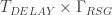
The time it takes to carry out a logical gate is decided each by 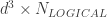

As a result of
At the very least they’re, till…………
FUNKY FEATURES OF PHOTONICS, PART II
However wait! There’s extra.
The second manner wherein distinctive options of photonics play havoc with the easy comparability to matter-based programs is within the thrilling risk of what we name an active-volume structure.
Just a few moments in the past I mentioned:
Even logical qubits that appear to not be a part of a gate in that point step bear a gate – the identification gate – as a result of they have to be saved error free whereas they “idle”. As such the whole variety of useful resource states consumed is simply
and that was true. Till not too long ago.
It seems that there’s a manner of eliminating nearly all of consumption of sources expended on idling qubits! That is achieved by some intelligent tips that make use of the potential of performing a restricted variety of non-nearest neighbor fusions between photons. It’s potential as a result of photons are usually not anyway caught in a single place, and they are often handed round readily with out interacting with different photons. (Their quantum crosstalk is strictly zero, they do actually appear to despise one another.)
What beforehand was a big quantity of useful resource states being consumed for “thumb-twiddling”, can as an alternative all be put to good use doing non-trivial computational gates. Right here is an easy quantum circuit with what we imply by the lively quantity highlighted:

Now, for any given computation the quantity of lively quantity will rely very a lot on what you might be computing. There are at all times many various circuits decomposing a given computation, some will use extra lively quantity than others. This makes it unimaginable to speak about “what’s the logical gate velocity” fully unbiased of issues in regards to the computation truly being carried out.
On this latest paper https://arxiv.org/abs/2306.08585 Daniel Litinski considers breaking elliptic curve cryptosystems on a quantum pc. Particularly, he considers what it could take to run the related model of Shor’s algorithm on a superconducting qubit structure with a 
He then compares fixing the identical downside on a machine with an lively quantity structure. Here’s a subset of his outcomes:

Recall that 


Now, this entire weblog put up is mainly about addressing confusions on the market relating to bodily versus computational timescales. So, for the sake of illustration, let me push a purely theoretical envelope: What if we will’t do the whole lot as quick as within the instance simply acknowledged? What if our price of whole useful resource state technology was 10 occasions slower, i.e. 

The quickest machine on this ridiculous machine would solely have to be a (very massive!) gradual optical swap working at 100KHz (as a result of chosen
To reiterate:
Regardless of all of the “bodily stuff happening” on this (hypothetical, active-volume) photonic machine working a lot slower than all of the “bodily stuff happening” within the (hypothetical, non-active-volume) superconducting qubit machine, we see the photonic machine can nonetheless do the specified computation 25 occasions sooner!
Hopefully the elemental murkiness of the titular query “what’s the logical gate velocity of a photonic quantum pc” is now clear! Put merely: Even when it did “basically run slower” (it gained’t), it could nonetheless be sooner. As a result of it has much less stuff to do. It’s value noting that the 25x enhance in velocity is clearly not primarily based on bodily timescales, however relatively on the environment friendly parallelization achieved by long-range connections within the photonic active-volume machine. If we had been to scale up the hypothetical 10-million-superconducting-qubit machine by an element of 25, it may probably additionally full computations 25 occasions sooner. Nevertheless, this might require a staggering 250 million bodily qubits or extra. In the end, absolutely the velocity restrict of quantum computations is about by the response time, which refers back to the time it takes to carry out a layer of single-qubit measurements and a few classical processing. Early-generation machines is not going to be restricted by this response time, though finally it is going to dictate the utmost velocity of a quantum computation. However even on this distant-future situation, the photonic method stays advantageous. As classical computation and communication velocity up past the microsecond vary, slower bodily measurements of matter-based qubits will hinder the response time, whereas quick single-photon detectors gained’t face the identical bottleneck.
In the usual photonic structure we noticed that 
With all this in thoughts it is usually value noting as an apart that optical fibers constituted of (costly!) unique glasses or with funky core buildings are theoretically calculated to be potential with as much as 100 occasions much less loss than standard fiber – due to this fact permitting for an equal scaling of
Clearly for pedagogical causes the above dialogue relies across the easiest approaches to logic in each customary and active-volume architectures, however extra detailed evaluation reveals that conclusions relating to whole computational time speedup persist even after identified optimizations for each approaches.
Now the explanation I referred to as the instance above a “ridiculous machine” is that even I’m not merciless sufficient to ask our engineers to assemble 350 billion useful resource state mills. Fewer useful resource state mills working sooner is fascinating from the attitude of each sweat and {dollars}.
We have now arrived then at a easy conclusion: what we actually have to know is “how briskly and at what scale can we generate useful resource states, with as massive a machine as we will afford to construct”.
HOW FAST COULD/SHOULD WE AIM TO DO RESOURCE STATE GENERATION?
On the planet of classical photonics – similar to that used for telecoms, LIDAR and so forth – very excessive speeds are sometimes thrown round: pulsed lasers and optical switches readily run at 100’s of GHz for instance. On the quantum facet, if we produce single photons by way of a probabilistic parametric course of then equally excessive repetition charges have been achieved. (It is because in such a course of there aren’t any timescale constraints set by atomic vitality ranges and so forth.) Off-the-shelf single photon avalanche photodiode detectors can depend photons at a number of GHz.
Looks as if we ought to be aiming to generate useful resource states at 10’s of GHz proper?
Effectively, sure, someday – one of many important causes I imagine the long-term way forward for quantum computing is finally photonic is due to the plain attainability of such timescales. [Two others: it’s the only sensible route to a large-scale room temperature machine; eventually there is only so much you can fit in a single cryostat, so ultimately any approach will converge to being a network of photonically linked machines].
In the actual world of quantum engineering there are a few causes to gradual issues down: (i) It relaxes {hardware} tolerances, because it makes it simpler to get issues like path lengths aligned, synchronization working, electronics working in straightforward regimes and so forth (ii) in an analogous solution to how we use interleaving throughout a computation to drastically scale back the variety of useful resource state mills we have to construct, we will additionally use (shorter than
Multiplexing is commonly misunderstood. The best way we produce the requisite photonic entanglement is probabilistic. Producing the entire 20-photon useful resource state in a single step, whereas potential, would have very low likelihood. The best way to obviate that is to cascade a few greater likelihood, intermediate, steps – choosing out successes (extra on this within the appendix). Whereas it has been identified because the seminal work of Knill, Laflamme and Milburn 20 years in the past that it is a smart factor to do, the impediment has at all times been the necessity for a excessive efficiency (quick, low loss) optical swap. Multiplexing introduces a brand new bodily “timescale of comfort” – mainly dictated by latencies of digital processing and sign transmission.
The temporary abstract due to this fact is: Yeah, the whole lot inner to creating useful resource states could be achieved at GHz charges, however a number of design flexibilities imply the speed of useful resource state technology is itself a parameter that ought to be tuned/optimized within the context of the entire machine, it isn’t constrained by basic quantum issues like interplay energies, relatively it’s constrained by the speeds of a bunch of purely classical stuff.
I don’t wish to go away the impression that technology of entangled photons can solely be achieved by way of the multistage probabilistic technique simply outlined. Utilizing quantum dots, for instance, individuals can already display technology of small photonic entangled states at GHz charges (see e.g. https://www.nature.com/articles/s41566-022-01152-2). Ultimately, direct technology of photonic entanglement from matter-based programs shall be how photonic quantum computer systems are constructed, and I ought to emphasize that its completely potential to make use of small useful resource states (say, 4 entangled photons) as an alternative of the 20 proposed above, so long as they’re extraordinarily clear and pure. In actual fact, because the dialogue above has hopefully made clear: for quantum computing approaches primarily based on basically gradual issues like atoms and ions, transduction of matter-based entanglement into photonic entanglement permits – by merely scaling to extra programs – evasion of the extraordinarily gradual logical gate speeds they are going to face if they don’t accomplish that.
Proper now, nonetheless, approaches primarily based on changing the entanglement of matter qubits into photonic entanglement are usually not almost clear sufficient, nor manufacturable at massive sufficient scales, to be suitable with utility-scale quantum computing. And our current technique of state technology by multiplexing has the additional advantage of decorrelating many error mechanisms which may in any other case be correlated if many photons originate from the identical machine.
So the place does all this go away us?
I wish to construct a helpful machine. Lets back-of-the-envelope what meaning photonically. Contemplate we goal a machine comprising (say) a minimum of 100 logical qubits able to billions of logical gates. (From desirous about lively quantity architectures I be taught that what I actually need is to provide as many “logical blocks” as potential, which might then be divvied up into computational/reminiscence/processing items in funky methods, so right here I’m actually simply spitballing an estimate to present you an concept).
Observing
and presuming 

None of those numbers ought to appear basically indigestible, although I don’t wish to understate the problem: all never-before-done large-scale engineering is extraordinarily onerous.
However whatever the regime we function in, logical gate speeds are usually not going to be the problem upon which photonics shall be discovered wanting.
REAL-WORLD QUANTUM COMPUTING DESIGN
Now, I do know this weblog is learn by numerous quantum physics college students. If you wish to affect the world, working in quantum computing actually is an effective way to do it. The muse of the whole lot spherical you within the trendy world was laid within the 40’s and 50’s when early mathematicians, pc scientists, physicists and engineers found out how we will compute classically. Right now you’ve a novel alternative to be a part of laying the muse of humanity’s quantum computing future. In fact, I need the perfect of you to work on a photonic method particularly (I’m additionally very completely happy to recommend locations for the worst of you to go work). Please recognize, due to this fact, that these last few paragraphs are my very biased – although happily completely appropriate – private perspective!
The broad options of the photonic machine described above – it’s a community of stuff to make useful resource states, stuff to fuse them, and a few interleaving modules, has been fastened now for a number of years (see the references).
As soon as we go down even only one stage of element, a myriad of very-much-not-independent questions come up: What’s the finest useful resource state? What collection of procedures is perfect for creating that state? What’s the finest underlying topological code to focus on? What fusion community can construct that code? What different issues (like lively quantity) can exploit the flexibility for photons to be simply nonlocally related? What sorts of encoding of quantum info into photonic states is finest? What interferometers generate essentially the most strong small entangled states? What procedures for systematically rising useful resource states from smaller entangled states are most strong or use the least quantity of {hardware}? How can we finest use measurements and classical feedforward/management to mitigate error accumulation?
These types of questions can’t be meaningfully addressed with out taking place to a different stage of element, one wherein we do appreciable modelling of the imperfect gadgets from which the whole lot shall be constructed – modelling that begins by detailed parameterization of about 40 part specs (ranging over issues like roughness of silicon photonic waveguide partitions, stability of built-in voltage drivers, precision of optical fiber slicing robots,….. Effectively, the checklist goes on and on). We then mannequin errors of subsystems constructed from these parts, confirm towards information, and proceed.
The upshot is none of those questions have distinctive solutions! There simply isn’t “one clearly finest code” and so forth. In actual fact the solutions can change considerably with even small variations in efficiency of the {hardware}. This opens a really wealthy design area, the place we will set up tradeoffs and select options that optimize all kinds of sensible {hardware} metrics.
In photonics there’s additionally significantly extra flexibility and alternative than with most approaches on the “quantum facet” of issues. That’s, the quantum facets of the sources, the quantum states we use for encoding even single qubits, the quantum states we must always goal for essentially the most strong entanglement, the topological quantum logical states we goal and so forth, are all “on the desk” so to talk.
Exploring the parameter area of potential machines to assemble, whereas staying absolutely related to part stage {hardware} efficiency, includes each having a really detailed simulation stack, and having sensible individuals to assist discover new and higher schemes to check within the simulations. It appears to me there are way more attention-grabbing avenues for impactful analysis than extra established approaches can declare. Proper now, on this planet, there are solely round 30 individuals engaged critically in that enterprise. It’s enjoyable. Maybe you must take part?
REFERENCES
A floor code quantum pc in silicon https://www.science.org/doi/10.1126/sciadv.1500707. Determine 4 is a transparent depiction of the circuits for performing a code cycle acceptable to a generic 2nd matter-based structure.
Fusion-based quantum computation https://arxiv.org/abs/2101.09310
Interleaving: Modular architectures for fault-tolerant photonic quantum computing https://arxiv.org/abs/2103.08612
Lively quantity: An structure for environment friendly fault-tolerant quantum computer systems with restricted non-local connections https://arxiv.org/abs/2211.15465
Learn how to compute a 256-bit elliptic curve personal key with solely 50 million Toffoli gates https://arxiv.org/abs/2211.15465
Conservation of Hassle: https://arxiv.org/abs/quant-ph/9902010
APPENDIX – A COMMON MISCONCEPTION
Here’s a frequent false impression: Present strategies of manufacturing ~20 photon entangled states succeed just a few occasions per second, so producing useful resource states for fusion-based quantum computing is many orders of magnitude away from the place it must be.
This false impression arises from contemplating experiments which produce photonic entangled states by way of single-shot spontaneous processes and extrapolating them incorrectly as having relevance to how useful resource states for photonic quantum computing are assembled.
Such single-shot experiments are hit by a “double whammy”. The primary whammy is that the experiments produce some very massive and messy state that solely has a tiny amplitude within the part of the specified entangled state. Thus, on every shot, even in preferrred circumstances, the likelihood of getting the specified state could be very, very small. As a result of billions of makes an attempt could be made every second (as talked about, working these gadgets at GHz speeds is simple) it does often happen. However solely a small variety of occasions per second.
The second whammy is that if you’re attempting to provide a 20-photon state, however every photon will get misplaced with likelihood 20%, then the likelihood of you detecting all of the photons – even in the event you stay in a department of the multiverse the place they’ve been produced – is diminished by an element of 
Now, photonic fusion-based quantum computing couldn’t be primarily based on such a entangled photon technology anyway, as a result of the manufacturing of the useful resource states must be heralded, whereas these experiments solely postselect onto the very tiny a part of the whole wavefunction with the specified entanglement. However allow us to put that apart, as a result of the 2 whammy’s may, in precept, be showstoppers for manufacturing of heralded useful resource states, and it’s helpful to know why they aren’t.
Think about you possibly can toss cash, and it is advisable generate 20 cash exhibiting Heads. Should you repeatedly toss all 20 cash concurrently till all of them come up heads you’d sometimes have to take action thousands and thousands of occasions earlier than you succeed. That is much more true if every coin additionally has a 20% likelihood of rolling off the desk (akin to photon loss). However in the event you can toss 20 cash, put aside (swap out!) those that got here up heads and re-toss the others, then after solely a small variety of steps you’ll have 20 cash all exhibiting heads. This massive hole is basically why the primary whammy shouldn’t be related: To generate a big photonic entangled state we start by probabilistically making an attempt to generate a bunch of small ones. We then choose out the success (multiplexing) and mix successes to (once more, probabilistically) generate a barely bigger entangled state. We repeat just a few steps of this. This risk has been appreciated for greater than twenty years, however hasn’t been achieved at scale but as a result of no person has had a ok optical swap till now.
The second whammy is taken care of the truth that for fault tolerant photonic fusion-based quantum computing there by no means is any have to make the useful resource state such that every one photons are assured to be there! The per-photon loss price could be excessive (in precept 10’s of p.c) – in reality the bigger the useful resource state being constructed the upper it’s allowed to be.
The upshot is that evaluating this technique of entangled photon technology with the strategies which are literally employed is considerably like a creation scientist claiming monkeys can not have advanced from micro organism, as a result of it’s all so unlikely for appropriate mutations to have occurred concurrently!
Acknowledgements
Very grateful to Mercedes Gimeno-Segovia, Daniel Litinski, Naomi Nickerson, Mike Nielsen and Pete Shadbolt for assist and suggestions.
[ad_2]